3D World Map: Air Connectivity
(Today all my team members were in office since the boss said he should be back today. He did not show up. But I am glad to see everyone in the new year!)
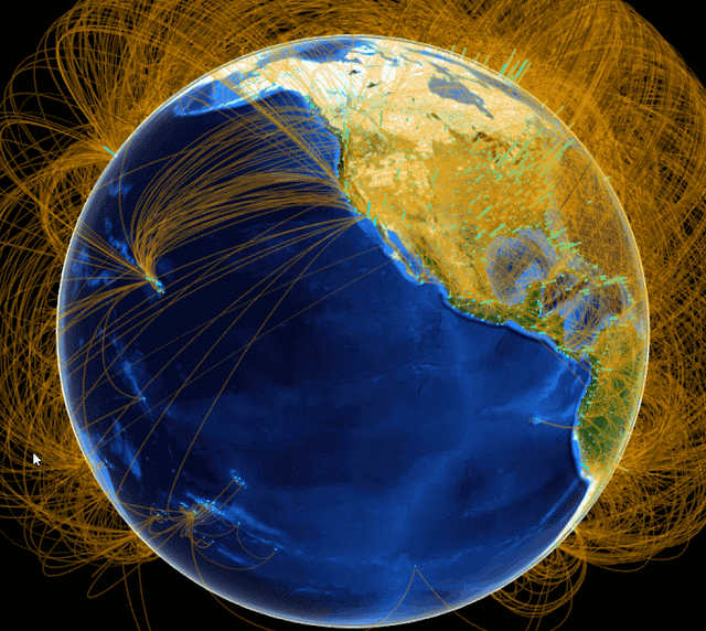
"Airport score" is a measurement created based on global airport network. It shows how centered each city is in the global air traffic network. In short, the airport score for each point on earth (or each city) is the sum product of airport weights and inverse distances to the point from all the airports. The airport weights are obtained through eigenvector centrality using a dataset of all the airline linkages in the world. I have already calculated all the scores but I was thinking over the new year how to visualize them. It turns out not so difficult:
I googled "3D world map in R" this morning and found an interesting blog by Mohit Singh, which I borrowed a lot. 3D world map can be done by the globejs function from R package threejs. The function can plot both points and arcs in the same time.
The centralized vector (weights of airports) was used to get the airport scores for global cities plotted in the last post. They were obtained before using eigen_centrality function from package igraph.
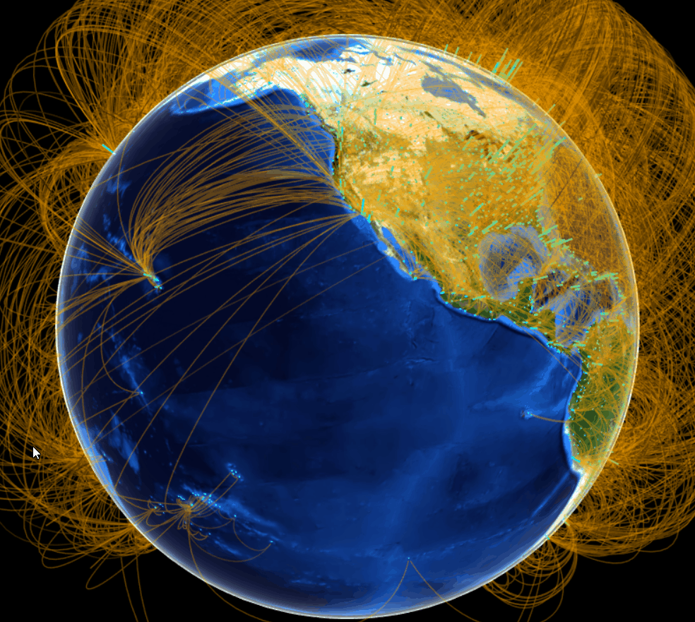
Updated 1.11.18: these are the new results updated in the Jan.11th post using a better dataset.
Top 10 airports by their relative importance (weights) in network

Top 10 cities in airport network by airport score calculated using the weights above

 ---
---
The post "Redo Airport Score" has more details on the methods.
Another post discussed how the geological distances were calculated.
"Airport score" is a measurement created based on global airport network. It shows how centered each city is in the global air traffic network. In short, the airport score for each point on earth (or each city) is the sum product of airport weights and inverse distances to the point from all the airports. The airport weights are obtained through eigenvector centrality using a dataset of all the airline linkages in the world. I have already calculated all the scores but I was thinking over the new year how to visualize them. It turns out not so difficult:
I googled "3D world map in R" this morning and found an interesting blog by Mohit Singh, which I borrowed a lot. 3D world map can be done by the globejs function from R package threejs. The function can plot both points and arcs in the same time.
Since my data are all the airport connections globally, it is a huge yarn ball.
I agree that orange seems to be a nice color for the arcs after trying many others.
 (The gif was created by capturing the screen directly using a free software "ScreenToGif".)
I agree that orange seems to be a nice color for the arcs after trying many others.
The extra contribution here is that I have also marked the importance of each airport (height of the blue dot) in the global network. This value can be calculated through eigenvector centrality. And in this case, it is actually not too different from counting the number of connections to each airport if turned into weights.
I used two datasets, one for the latitude and longitude of the points to be shown (air3), one for the arcs to be drawn (air2). Dataset "air2" has 4 columns (3:6 in my case) to supply: lat and long for the starting point, and lat and long for the endpoint for each arc. My data were also obtained from open flights.
library("readxl")
air2 <- read_excel("D:/NYU Marron/Data/airport_route3.xlsx", sheet = "Sheet1")
air2 <- as.data.frame(air2)
# The loaded data contains the sources and destinations of arcs
head(air2)
## # Source Destination SourceLat SourceLong DestLat DestLong
## 1 794 AAE ALG 36.8222 7.80917 36.69100 3.215410
## 2 794 AAE CDG 36.8222 7.80917 49.01280 2.550000
## 3 794 AAE IST 36.8222 7.80917 40.97690 28.814600
## 4 794 AAE LYS 36.8222 7.80917 45.72556 5.081111
## 5 794 AAE MRS 36.8222 7.80917 43.43927 5.221424
## 6 794 AAE ORN 36.8222 7.80917 35.62390 -0.621183# Get airport names and their location without repeat
# A little bit complicated as some airport only appear in the Source or Destination
# And I shall get the names for all the airports in the dataset
air2_sub <- air2[c("Source","Destination")]
air_source <- air2[c("Source", "SourceLat", "SourceLong")]
air_dest <- air2[c("Destination", "DestLat", "DestLong")]
names(air_source) <- names(air_dest) <- c("Source","SourceLat","SourceLong")
air2_long <- rbind(air_source, air_dest)
air2_long$Source <- as.factor(air2_long$Source)
# remove duplciate to get unique list of airports
air2_nodup <- air2_long[!duplicated(air2_long$Source),]
head(air2_nodup)## Source SourceLat SourceLong
## 1 AAE 36.82220 7.809170
## 10 AAL 57.09276 9.849243
## 30 AAN 24.26170 55.609200
## 32 AAQ 45.00210 37.347301
## 35 AAR 56.30000 10.619000
## 43 AAT 47.86667 88.116667The centralized vector (weights of airports) was used to get the airport scores for global cities plotted in the last post. They were obtained before using eigen_centrality function from package igraph.
# Create weights by eigen_centrality
library("igraph")
air_graph <- graph.data.frame(air2_sub)
# obtain the vector
air2_Vector <- eigen_centrality(air_graph)$vector
# air2_Vector is named num, use names() to extract the airport names
# so later it can merge with air2_nodup to generate air3.
air2_Vector_Data <- data.frame(names(air2_Vector),air2_Vector)
names(air2_Vector_Data) <- c("Source","V")
air2_Vector_Data$Source <- as.factor(air2_Vector_Data$Source)
# air3 contains airport name, weights, latitutde and longitude
air3 <- merge(air2_Vector_Data, air2_nodup, by="Source" )
head(air3)## Source V SourceLat SourceLong
## 1 AAE 0.0085039898 36.82220 7.809170
## 2 AAL 0.0232751327 57.09276 9.849243
## 3 AAN 0.0002135457 24.26170 55.609200
## 4 AAQ 0.0023122646 45.00210 37.347301
## 5 AAR 0.0053742630 56.30000 10.619000
## 6 AAT 0.0010224887 47.86667 88.116667# Plot all the cities and arcs
library("threejs")
library("maps")
# Get the image of the globe - NASA
earth_image <- "http://eoimages.gsfc.nasa.gov/images/imagerecords/73000/73909/world.topo.bathy.200412.3x5400x2700.jpg"
#Display the data on the globe
globejs(
img = earth_image,
# points
lat = air3$SourceLat, long = air3$SourceLong, value=air3$V*100, # height
# arcs
arcs = air2[, 4:7], arcsOpacity = 0.20, arcsHeight = 0.5, arcsLwd = 1,
arcsColor = "orange", atmosphere = TRUE,
height = 800, width = 800, bg = "black"
)Updated 1.11.18: these are the new results updated in the Jan.11th post using a better dataset.
Top 10 airports by their relative importance (weights) in network


A better shot of the yarn ball:

The post "Redo Airport Score" has more details on the methods.
Another post discussed how the geological distances were calculated.


Comments