Modeling of Slums: Model Selection using Lasso and Best Subset
Model Selection using Lasso and Best Subset
Model Selection using Lasso and Best Subset

-
- 1. Linear regression model with Lasso feature selection
- 2. Linear regression model with Best Subset selection
- 3. Random Forest
- Conclusion
- Complete Code
I will give a short introduction to statistical learning and modeling, apply feature (variable) selection using Best Subset and Lasso. The dependent variable to model is Share_Temporary: Share of Temporary Structure in Slums. The independent variables are monitoring indicators like water, sanitation, housing conditions and overcrowding. Each of the 600 observations used is a slum settlement. I will also compare the results to Random Forest in the end.
- 1. Linear regression model with Lasso feature selection
- 2. Linear regression model with Best Subset selection
- 3. Random Forest
- Conclusion
- Complete Code
I will give a short introduction to statistical learning and modeling, apply feature (variable) selection using Best Subset and Lasso. The dependent variable to model is
Share_Temporary: Share of Temporary Structure in Slums. The independent variables are monitoring indicators like water, sanitation, housing conditions and overcrowding. Each of the 600 observations used is a slum settlement. I will also compare the results to Random Forest in the end.Prediction and Inference
-
The two main motivations for statistical modeling (e.g. run a linear regression model) are prediction (to predict) and inference (to explain).
- Prediction usually needs cross-validation, which fits the model on a training dataset. By checking model’s performance on a separate testing dataset, we know how good the model will be when facing new data in the future.
- Inference tries to understand the relationship among variables, and the effect of the predictor on the dependent variable after controlling for the others variables. Usually, we hope the predictors used fit significantly into the model and the variables used should make sense in the real world.
The complete codes are attached in the end.
Prepare dataset
-
The dataset is cleaned, divided into training and testing, and is prepared in both matrix and data frame format as needed for different applications.
There are 50 features to select from. The Y_train and Y_test have only one column (the dependent variable).
dim(mydata4)
## [1] 598 51
dim(X_train)
## [1] 358 50
dim(X_test)
## [1] 240 50
The dataset is cleaned, divided into training and testing, and is prepared in both matrix and data frame format as needed for different applications.
There are 50 features to select from. The
There are 50 features to select from. The
Y_train and Y_test have only one column (the dependent variable).dim(mydata4)## [1] 598 51dim(X_train)## [1] 358 50dim(X_test)## [1] 240 501. Linear regression model with Lasso feature selection
-
Use library
glmnet.
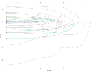
Lasso is a shrinkage approach for feature selection. The tuning parameter lambda is the magnitudes of penalty. An increasing penalty shrinks coefficients towards zero. We see in the figure below as lambda increases, more and more coefficients merge to zero (horizontal line in the middle).
 We use cross-validation to choose the lambda, and corresponding variables used to fit the linear regression.
* The dotted line on the left is lambda.min, the lambda that generates the lowest MSE in the testing dataset. The dotted line on the right is lambda.1se, its corresponding MSE is not the lowest but acceptable, and it has even fewer features in the model. We use lambda.1se in our case.
# Use cross-validation to select the lambda
cv_lasso <- cv.glmnet(X_train, Y_train, alpha = 1) # Lasso regression
plot.cv.glmnet(cv_lasso)

# lambda selected by 1se rule
(best_lam <- cv_lasso$lambda.1se)
## [1] 0.02664
# Check prediction error in the testing dataset
lasso_pred <- predict(lasso_mod, s = best_lam, newx = X_test)
# The Mean squared error (MSE)
(MSE_Lasso <- mean((lasso_pred - Y_test)^2))
## [1] 0.06833
- The regression model for the selected lambda (lasso). We extract the coefficients from the selected model and run a linear regression.
- The model has used 16 variables.
# coef_table is class 'dgCMatrix' of the selected coefficients for each lambda
coef_table <- coef(cv_lasso, s = cv_lasso$lambda.1se)
# Because there is the intercept on the first column, we use [coef_table@i + 1] to extract the names of coefficients (Dimnames) from class 'dgCMatrix', and [-1] in the end
var_list <- unlist(coef_table@Dimnames[[1]][coef_table@i + 1])
sdi_sub <- mydata4[c(coef_table@Dimnames[[1]][coef_table@i + 1], "Share_Temporary")[-1]]
reg.chosen1 <- lm(data = sdi_sub, Share_Temporary~.)
summary(reg.chosen1)
##
## Call:
## lm(formula = Share_Temporary ~ ., data = sdi_sub)
##
## Residuals:
## Min 1Q Median 3Q Max
## -0.6581 -0.1713 -0.0154 0.1722 0.6496
##
## Coefficients:
## Estimate Std. Error t value
## (Intercept) 6.07e-01 2.97e-02 20.43
## CC11_Population_Estimate -6.56e-07 2.40e-07 -2.73
## B14__declared_legal_protected 8.94e-02 2.71e-02 3.30
## B14__resettled -1.52e-01 2.96e-02 -5.14
## Eviction_Threats 1.09e-01 2.22e-02 4.88
## C13__no_rent 1.25e-01 5.77e-02 2.16
## FF1_8_Water_Sourcesshared_taps -1.19e-01 3.09e-02 -3.86
## FF1_8_Water_Sourceswells -7.86e-02 2.16e-02 -3.64
## FF1_8_Water_Sourcesdams -2.79e-02 4.49e-02 -0.62
## FF1_8_Water_Sourceswater_tankers -1.15e-01 3.59e-02 -3.19
## FF11_Water_MonthlyCost -4.19e-06 6.37e-07 -6.59
## GG1_Sewer_Line 4.93e-02 2.41e-02 2.04
## GG7_10_Toilet_Typescommunal_toilets -7.62e-02 2.66e-02 -2.86
## DD1_Location_Problemscanal -8.59e-02 2.67e-02 -3.21
## DD1_Location_Problemsslope -1.01e-01 2.21e-02 -4.57
## DD1_Location_Problemsflood_prone_area -8.41e-02 2.21e-02 -3.81
## DD1_Location_Problemswater_body -5.02e-02 2.73e-02 -1.84
## Pr(>|t|)
## (Intercept) < 2e-16 ***
## CC11_Population_Estimate 0.00651 **
## B14__declared_legal_protected 0.00103 **
## B14__resettled 3.7e-07 ***
## Eviction_Threats 1.4e-06 ***
## C13__no_rent 0.03114 *
## FF1_8_Water_Sourcesshared_taps 0.00013 ***
## FF1_8_Water_Sourceswells 0.00029 ***
## FF1_8_Water_Sourcesdams 0.53412
## FF1_8_Water_Sourceswater_tankers 0.00148 **
## FF11_Water_MonthlyCost 1.0e-10 ***
## GG1_Sewer_Line 0.04180 *
## GG7_10_Toilet_Typescommunal_toilets 0.00439 **
## DD1_Location_Problemscanal 0.00140 **
## DD1_Location_Problemsslope 5.9e-06 ***
## DD1_Location_Problemsflood_prone_area 0.00015 ***
## DD1_Location_Problemswater_body 0.06698 .
## ---
## Signif. codes: 0 '***' 0.001 '**' 0.01 '*' 0.05 '.' 0.1 ' ' 1
##
## Residual standard error: 0.243 on 581 degrees of freedom
## Multiple R-squared: 0.557, Adjusted R-squared: 0.545
## F-statistic: 45.7 on 16 and 581 DF, p-value: <2e-16
If we want a model for explanatory purpose, we can remove some insignificant predictors. This gives the basic model that we can further modify to show the relationships describing the dependent variable Share_Temporary.
- The most powerful (useful) predictors include
Water_MonthlyCost, Water_Sources: shared_taps, Resettled Housing and Eviction Threats. For these variables, higher values or binary variables being Yes are associated with fewer temporary structures in slums.
- Examining the shared selections from different approaches gives us a sense of what are the most important variables for inference.
##
## Call:
## lm(formula = Share_Temporary ~ FF11_Water_MonthlyCost + FF1_8_Water_Sourcesshared_taps +
##     B14__resettled + FF1_8_Water_Sourceswells + DD1_Location_Problemsslope +
##     DD1_Location_Problemsflood_prone_area + Eviction_Threats +
##     GG1_Sewer_Line + DD1_Location_Problemscanal + C13__no_rent,
##     data = sdi)
##
## Residuals:
##     Min      1Q  Median      3Q     Max
## -0.6978 -0.1841 -0.0163  0.1978  0.7921
##
## Coefficients:
##                                        Estimate Std. Error t value
## (Intercept)                            6.64e-01   2.37e-02   27.96
## FF11_Water_MonthlyCost                -5.38e-06   5.82e-07   -9.25
## FF1_8_Water_Sourcesshared_taps        -2.01e-01   2.68e-02   -7.50
## B14__resettled                        -1.56e-01   2.56e-02   -6.07
## FF1_8_Water_Sourceswells              -1.26e-01   2.01e-02   -6.25
## DD1_Location_Problemsslope            -1.13e-01   2.11e-02   -5.38
## DD1_Location_Problemsflood_prone_area -8.54e-02   2.04e-02   -4.19
## Eviction_Threats                       7.57e-02   2.07e-02    3.65
## GG1_Sewer_Line                         8.21e-02   2.24e-02    3.66
## DD1_Location_Problemscanal            -7.50e-02   2.56e-02   -2.93
## C13__no_rent                           1.41e-01   5.11e-02    2.76
##                                       Pr(>|t|)
## (Intercept)                            < 2e-16 ***
## FF11_Water_MonthlyCost                 < 2e-16 ***
## FF1_8_Water_Sourcesshared_taps         1.8e-13 ***
## B14__resettled                         2.0e-09 ***
## FF1_8_Water_Sourceswells               7.0e-10 ***
## DD1_Location_Problemsslope             1.0e-07 ***
## DD1_Location_Problemsflood_prone_area  3.1e-05 ***
## Eviction_Threats                       0.00028 ***
## GG1_Sewer_Line                         0.00027 ***
## DD1_Location_Problemscanal             0.00351 **
## C13__no_rent                           0.00595 **
## ---
## Signif. codes:  0 '***' 0.001 '**' 0.01 '*' 0.05 '.' 0.1 ' ' 1
##
## Residual standard error: 0.262 on 754 degrees of freedom
##   (210 observations deleted due to missingness)
## Multiple R-squared:  0.507,  Adjusted R-squared:  0.501
## F-statistic: 77.6 on 10 and 754 DF,  p-value: <2e-16
- The relative importance of coefficients by showing standardized regression coefficients in decreasing order of their absolute values.
coef_table2 <- data.frame(b = reg.chosen2$coefficients, stb = c(0, lm.beta(reg.chosen2)))
coef_table2[order(abs(coef_table2$stb), decreasing = T),]
##                                                b      stb
## FF11_Water_MonthlyCost                -5.384e-06 -0.28553
## FF1_8_Water_Sourcesshared_taps        -2.010e-01 -0.20358
## B14__resettled                        -1.556e-01 -0.19021
## FF1_8_Water_Sourceswells              -1.255e-01 -0.16851
## DD1_Location_Problemsslope            -1.135e-01 -0.15231
## DD1_Location_Problemsflood_prone_area -8.539e-02 -0.11400
## Eviction_Threats                       7.566e-02  0.10084
## GG1_Sewer_Line                         8.211e-02  0.09914
## DD1_Location_Problemscanal            -7.501e-02 -0.08267
## C13__no_rent                           1.409e-01  0.07259
## (Intercept)                            6.638e-01  0.00000
Use library
Lasso is a shrinkage approach for feature selection. The tuning parameter lambda is the magnitudes of penalty. An increasing penalty shrinks coefficients towards zero. We see in the figure below as lambda increases, more and more coefficients merge to zero (horizontal line in the middle).
glmnet.Lasso is a shrinkage approach for feature selection. The tuning parameter lambda is the magnitudes of penalty. An increasing penalty shrinks coefficients towards zero. We see in the figure below as lambda increases, more and more coefficients merge to zero (horizontal line in the middle).
We use cross-validation to choose the lambda, and corresponding variables used to fit the linear regression.
* The dotted line on the left is lambda.min, the lambda that generates the lowest MSE in the testing dataset. The dotted line on the right is lambda.1se, its corresponding MSE is not the lowest but acceptable, and it has even fewer features in the model. We use
* The dotted line on the left is lambda.min, the lambda that generates the lowest MSE in the testing dataset. The dotted line on the right is lambda.1se, its corresponding MSE is not the lowest but acceptable, and it has even fewer features in the model. We use
lambda.1se in our case.# Use cross-validation to select the lambda
cv_lasso <- cv.glmnet(X_train, Y_train, alpha = 1) # Lasso regression
plot.cv.glmnet(cv_lasso)
# lambda selected by 1se rule
(best_lam <- cv_lasso$lambda.1se)## [1] 0.02664# Check prediction error in the testing dataset
lasso_pred <- predict(lasso_mod, s = best_lam, newx = X_test)
# The Mean squared error (MSE)
(MSE_Lasso <- mean((lasso_pred - Y_test)^2))## [1] 0.06833- The regression model for the selected lambda (lasso). We extract the coefficients from the selected model and run a linear regression.
- The model has used 16 variables.
# coef_table is class 'dgCMatrix' of the selected coefficients for each lambda
coef_table <- coef(cv_lasso, s = cv_lasso$lambda.1se)
# Because there is the intercept on the first column, we use [coef_table@i + 1] to extract the names of coefficients (Dimnames) from class 'dgCMatrix', and [-1] in the end
var_list <- unlist(coef_table@Dimnames[[1]][coef_table@i + 1])
sdi_sub <- mydata4[c(coef_table@Dimnames[[1]][coef_table@i + 1], "Share_Temporary")[-1]]
reg.chosen1 <- lm(data = sdi_sub, Share_Temporary~.)
summary(reg.chosen1)##
## Call:
## lm(formula = Share_Temporary ~ ., data = sdi_sub)
##
## Residuals:
## Min 1Q Median 3Q Max
## -0.6581 -0.1713 -0.0154 0.1722 0.6496
##
## Coefficients:
## Estimate Std. Error t value
## (Intercept) 6.07e-01 2.97e-02 20.43
## CC11_Population_Estimate -6.56e-07 2.40e-07 -2.73
## B14__declared_legal_protected 8.94e-02 2.71e-02 3.30
## B14__resettled -1.52e-01 2.96e-02 -5.14
## Eviction_Threats 1.09e-01 2.22e-02 4.88
## C13__no_rent 1.25e-01 5.77e-02 2.16
## FF1_8_Water_Sourcesshared_taps -1.19e-01 3.09e-02 -3.86
## FF1_8_Water_Sourceswells -7.86e-02 2.16e-02 -3.64
## FF1_8_Water_Sourcesdams -2.79e-02 4.49e-02 -0.62
## FF1_8_Water_Sourceswater_tankers -1.15e-01 3.59e-02 -3.19
## FF11_Water_MonthlyCost -4.19e-06 6.37e-07 -6.59
## GG1_Sewer_Line 4.93e-02 2.41e-02 2.04
## GG7_10_Toilet_Typescommunal_toilets -7.62e-02 2.66e-02 -2.86
## DD1_Location_Problemscanal -8.59e-02 2.67e-02 -3.21
## DD1_Location_Problemsslope -1.01e-01 2.21e-02 -4.57
## DD1_Location_Problemsflood_prone_area -8.41e-02 2.21e-02 -3.81
## DD1_Location_Problemswater_body -5.02e-02 2.73e-02 -1.84
## Pr(>|t|)
## (Intercept) < 2e-16 ***
## CC11_Population_Estimate 0.00651 **
## B14__declared_legal_protected 0.00103 **
## B14__resettled 3.7e-07 ***
## Eviction_Threats 1.4e-06 ***
## C13__no_rent 0.03114 *
## FF1_8_Water_Sourcesshared_taps 0.00013 ***
## FF1_8_Water_Sourceswells 0.00029 ***
## FF1_8_Water_Sourcesdams 0.53412
## FF1_8_Water_Sourceswater_tankers 0.00148 **
## FF11_Water_MonthlyCost 1.0e-10 ***
## GG1_Sewer_Line 0.04180 *
## GG7_10_Toilet_Typescommunal_toilets 0.00439 **
## DD1_Location_Problemscanal 0.00140 **
## DD1_Location_Problemsslope 5.9e-06 ***
## DD1_Location_Problemsflood_prone_area 0.00015 ***
## DD1_Location_Problemswater_body 0.06698 .
## ---
## Signif. codes: 0 '***' 0.001 '**' 0.01 '*' 0.05 '.' 0.1 ' ' 1
##
## Residual standard error: 0.243 on 581 degrees of freedom
## Multiple R-squared: 0.557, Adjusted R-squared: 0.545
## F-statistic: 45.7 on 16 and 581 DF, p-value: <2e-16
If we want a model for explanatory purpose, we can remove some insignificant predictors. This gives the basic model that we can further modify to show the relationships describing the dependent variable
Share_Temporary.- The most powerful (useful) predictors include
Water_MonthlyCost,Water_Sources: shared_taps,Resettled HousingandEviction Threats. For these variables, higher values or binary variables being Yes are associated with fewer temporary structures in slums. - Examining the shared selections from different approaches gives us a sense of what are the most important variables for inference.
##
## Call:
## lm(formula = Share_Temporary ~ FF11_Water_MonthlyCost + FF1_8_Water_Sourcesshared_taps +
## B14__resettled + FF1_8_Water_Sourceswells + DD1_Location_Problemsslope +
## DD1_Location_Problemsflood_prone_area + Eviction_Threats +
## GG1_Sewer_Line + DD1_Location_Problemscanal + C13__no_rent,
## data = sdi)
##
## Residuals:
## Min 1Q Median 3Q Max
## -0.6978 -0.1841 -0.0163 0.1978 0.7921
##
## Coefficients:
## Estimate Std. Error t value
## (Intercept) 6.64e-01 2.37e-02 27.96
## FF11_Water_MonthlyCost -5.38e-06 5.82e-07 -9.25
## FF1_8_Water_Sourcesshared_taps -2.01e-01 2.68e-02 -7.50
## B14__resettled -1.56e-01 2.56e-02 -6.07
## FF1_8_Water_Sourceswells -1.26e-01 2.01e-02 -6.25
## DD1_Location_Problemsslope -1.13e-01 2.11e-02 -5.38
## DD1_Location_Problemsflood_prone_area -8.54e-02 2.04e-02 -4.19
## Eviction_Threats 7.57e-02 2.07e-02 3.65
## GG1_Sewer_Line 8.21e-02 2.24e-02 3.66
## DD1_Location_Problemscanal -7.50e-02 2.56e-02 -2.93
## C13__no_rent 1.41e-01 5.11e-02 2.76
## Pr(>|t|)
## (Intercept) < 2e-16 ***
## FF11_Water_MonthlyCost < 2e-16 ***
## FF1_8_Water_Sourcesshared_taps 1.8e-13 ***
## B14__resettled 2.0e-09 ***
## FF1_8_Water_Sourceswells 7.0e-10 ***
## DD1_Location_Problemsslope 1.0e-07 ***
## DD1_Location_Problemsflood_prone_area 3.1e-05 ***
## Eviction_Threats 0.00028 ***
## GG1_Sewer_Line 0.00027 ***
## DD1_Location_Problemscanal 0.00351 **
## C13__no_rent 0.00595 **
## ---
## Signif. codes: 0 '***' 0.001 '**' 0.01 '*' 0.05 '.' 0.1 ' ' 1
##
## Residual standard error: 0.262 on 754 degrees of freedom
## (210 observations deleted due to missingness)
## Multiple R-squared: 0.507, Adjusted R-squared: 0.501
## F-statistic: 77.6 on 10 and 754 DF, p-value: <2e-16- The relative importance of coefficients by showing standardized regression coefficients in decreasing order of their absolute values.
coef_table2 <- data.frame(b = reg.chosen2$coefficients, stb = c(0, lm.beta(reg.chosen2)))
coef_table2[order(abs(coef_table2$stb), decreasing = T),]## b stb
## FF11_Water_MonthlyCost -5.384e-06 -0.28553
## FF1_8_Water_Sourcesshared_taps -2.010e-01 -0.20358
## B14__resettled -1.556e-01 -0.19021
## FF1_8_Water_Sourceswells -1.255e-01 -0.16851
## DD1_Location_Problemsslope -1.135e-01 -0.15231
## DD1_Location_Problemsflood_prone_area -8.539e-02 -0.11400
## Eviction_Threats 7.566e-02 0.10084
## GG1_Sewer_Line 8.211e-02 0.09914
## DD1_Location_Problemscanal -7.501e-02 -0.08267
## C13__no_rent 1.409e-01 0.07259
## (Intercept) 6.638e-01 0.000002. Best Subset
-
Use library
leaps.
Best subset is a subset selection approach for feature selection. Not like stepwise or forward selection, best subset run the regressions for all the possible combinations of variables. For 30 predictors to select, there would be 2^30 = 1,073,741,824 over one billion models to check. Since I select from 49 predictors but set the maximum size of subsets to be 25, there are C(49,25) + C(49,24) + ...+ C(49,0) = 345 trillion models to check, which took me hours (3 hours this time, sometimes faster, 1 hour) in R using leaps library (right, still too fast to be true). But it was done in three seconds in SAS (using proc reg, Mallows's Cp). As I discussed in my later post, both R and SAS apply the branch and bound algorithm, which speeds up the calculation. It won't be possible to scan all the possible models.
- The tuning parameter is to decide how many predictors to use
- If without cross-validation we can use the traditional way to choose model: Adjusted R-squared, Cp(AIC), or BIC.
time_now <- Sys.time()
nv_max <- 25
fit_s <- regsubsets(Share_Temporary~., data_train,
                    really.big = T, nbest=1, nvmax = nv_max
)
## Reordering variables and trying again:
Sys.time() - time_now
## Time difference of 3.149 hours
 As shown above, if we choose the number of variables by Mallows's CP, there are 24 variables (SAS chooses 23 use CP). BIC indicates 11 variables. Here we choose the number of features by checking the error rates of models on the testing dataset:
- The selected number of features is 17
(val_err_min <- which.min(val.errors))
## [1] 17
- MSE:
(MSE_best.subset <- val.errors[val_err_min])
## [1] 0.07205
- The regression model selected using best subset:
- This model has 17 predictors. 9 of the variables are the same as the model selected by the Lasso.
##
## Call:
## lm(formula = Share_Temporary ~ ., data = sdi_sub2)
##
## Residuals:
##     Min      1Q  Median      3Q     Max
## -0.7473 -0.1739 -0.0308  0.1910  0.7606
##
## Coefficients:
##                                        Estimate Std. Error t value
## (Intercept)                            7.38e-01   5.36e-02   13.77
## B14__declared_legal_protected          7.41e-02   2.85e-02    2.60
## B14__resettled                        -1.82e-01   3.25e-02   -5.59
## Eviction_Threats                       1.38e-01   3.41e-02    4.06
## EE2A_Current_Eviction_Threat          -1.42e-02   3.46e-02   -0.41
## FF1_8_Water_Sourcesshared_taps        -1.37e-01   3.21e-02   -4.28
## FF1_8_Water_Sourcesdams               -9.24e-02   4.55e-02   -2.03
## FF1_8_Water_Sourcessprings            -8.78e-02   2.99e-02   -2.93
## FF1_8_Water_Sourcesrivers             -3.73e-02   3.84e-02   -0.97
## FF1_8_Water_Sourceswater_tankers      -1.43e-01   3.69e-02   -3.89
## FF11_Water_MonthlyCost                -4.79e-06   6.63e-07   -7.23
## FF12_Water_CollectionTime30_minutes    2.08e-02   3.22e-02    0.65
## GG7_10_Toilet_Typesindividual_toilets -6.26e-02   3.05e-02   -2.05
## DD1_Location_Problemscanal            -1.06e-01   2.76e-02   -3.84
## DD1_Location_Problemsflood_prone_area -1.25e-01   2.22e-02   -5.63
## DD1_Location_Problemsgarbage_dump      2.37e-03   2.35e-02    0.10
## DD1_Location_Problemsroad_side        -1.39e-02   2.35e-02   -0.59
## JJ1_Electricity_Availableyes          -1.22e-01   4.16e-02   -2.93
##                                       Pr(>|t|)
## (Intercept)                            < 2e-16 ***
## B14__declared_legal_protected          0.00955 **
## B14__resettled                         3.6e-08 ***
## Eviction_Threats                       5.7e-05 ***
## EE2A_Current_Eviction_Threat           0.68097
## FF1_8_Water_Sourcesshared_taps         2.2e-05 ***
## FF1_8_Water_Sourcesdams                0.04258 *
## FF1_8_Water_Sourcessprings             0.00348 **
## FF1_8_Water_Sourcesrivers              0.33241
## FF1_8_Water_Sourceswater_tankers       0.00011 ***
## FF11_Water_MonthlyCost                 1.5e-12 ***
## FF12_Water_CollectionTime30_minutes    0.51812
## GG7_10_Toilet_Typesindividual_toilets  0.04054 *
## DD1_Location_Problemscanal             0.00014 ***
## DD1_Location_Problemsflood_prone_area  2.8e-08 ***
## DD1_Location_Problemsgarbage_dump      0.91970
## DD1_Location_Problemsroad_side         0.55452
## JJ1_Electricity_Availableyes           0.00349 **
## ---
## Signif. codes:  0 '***' 0.001 '**' 0.01 '*' 0.05 '.' 0.1 ' ' 1
##
## Residual standard error: 0.253 on 580 degrees of freedom
## Multiple R-squared:  0.523,  Adjusted R-squared:  0.509
## F-statistic: 37.3 on 17 and 580 DF,  p-value: <2e-16
Use library
Best subset is a subset selection approach for feature selection. Not like stepwise or forward selection, best subset run the regressions for all the possible combinations of variables. For 30 predictors to select, there would be 2^30 = 1,073,741,824 over one billion models to check. Since I select from 49 predictors but set the maximum size of subsets to be 25, there are C(49,25) + C(49,24) + ...+ C(49,0) = 345 trillion models to check, which took me hours (3 hours this time, sometimes faster, 1 hour) in R using
leaps.Best subset is a subset selection approach for feature selection. Not like stepwise or forward selection, best subset run the regressions for all the possible combinations of variables. For 30 predictors to select, there would be 2^30 = 1,073,741,824 over one billion models to check. Since I select from 49 predictors but set the maximum size of subsets to be 25, there are C(49,25) + C(49,24) + ...+ C(49,0) = 345 trillion models to check, which took me hours (3 hours this time, sometimes faster, 1 hour) in R using
leaps library (right, still too fast to be true). But it was done in three seconds in SAS (using proc reg, Mallows's Cp). As I discussed in my later post, both R and SAS apply the branch and bound algorithm, which speeds up the calculation. It won't be possible to scan all the possible models.- The tuning parameter is to decide how many predictors to use
- If without cross-validation we can use the traditional way to choose model: Adjusted R-squared, Cp(AIC), or BIC.
time_now <- Sys.time()
nv_max <- 25
fit_s <- regsubsets(Share_Temporary~., data_train,
really.big = T, nbest=1, nvmax = nv_max
)## Reordering variables and trying again:Sys.time() - time_now## Time difference of 3.149 hours- The selected number of features is 17
(val_err_min <- which.min(val.errors))## [1] 17- MSE:
(MSE_best.subset <- val.errors[val_err_min])## [1] 0.07205- The regression model selected using best subset:
- This model has 17 predictors. 9 of the variables are the same as the model selected by the Lasso.
##
## Call:
## lm(formula = Share_Temporary ~ ., data = sdi_sub2)
##
## Residuals:
## Min 1Q Median 3Q Max
## -0.7473 -0.1739 -0.0308 0.1910 0.7606
##
## Coefficients:
## Estimate Std. Error t value
## (Intercept) 7.38e-01 5.36e-02 13.77
## B14__declared_legal_protected 7.41e-02 2.85e-02 2.60
## B14__resettled -1.82e-01 3.25e-02 -5.59
## Eviction_Threats 1.38e-01 3.41e-02 4.06
## EE2A_Current_Eviction_Threat -1.42e-02 3.46e-02 -0.41
## FF1_8_Water_Sourcesshared_taps -1.37e-01 3.21e-02 -4.28
## FF1_8_Water_Sourcesdams -9.24e-02 4.55e-02 -2.03
## FF1_8_Water_Sourcessprings -8.78e-02 2.99e-02 -2.93
## FF1_8_Water_Sourcesrivers -3.73e-02 3.84e-02 -0.97
## FF1_8_Water_Sourceswater_tankers -1.43e-01 3.69e-02 -3.89
## FF11_Water_MonthlyCost -4.79e-06 6.63e-07 -7.23
## FF12_Water_CollectionTime30_minutes 2.08e-02 3.22e-02 0.65
## GG7_10_Toilet_Typesindividual_toilets -6.26e-02 3.05e-02 -2.05
## DD1_Location_Problemscanal -1.06e-01 2.76e-02 -3.84
## DD1_Location_Problemsflood_prone_area -1.25e-01 2.22e-02 -5.63
## DD1_Location_Problemsgarbage_dump 2.37e-03 2.35e-02 0.10
## DD1_Location_Problemsroad_side -1.39e-02 2.35e-02 -0.59
## JJ1_Electricity_Availableyes -1.22e-01 4.16e-02 -2.93
## Pr(>|t|)
## (Intercept) < 2e-16 ***
## B14__declared_legal_protected 0.00955 **
## B14__resettled 3.6e-08 ***
## Eviction_Threats 5.7e-05 ***
## EE2A_Current_Eviction_Threat 0.68097
## FF1_8_Water_Sourcesshared_taps 2.2e-05 ***
## FF1_8_Water_Sourcesdams 0.04258 *
## FF1_8_Water_Sourcessprings 0.00348 **
## FF1_8_Water_Sourcesrivers 0.33241
## FF1_8_Water_Sourceswater_tankers 0.00011 ***
## FF11_Water_MonthlyCost 1.5e-12 ***
## FF12_Water_CollectionTime30_minutes 0.51812
## GG7_10_Toilet_Typesindividual_toilets 0.04054 *
## DD1_Location_Problemscanal 0.00014 ***
## DD1_Location_Problemsflood_prone_area 2.8e-08 ***
## DD1_Location_Problemsgarbage_dump 0.91970
## DD1_Location_Problemsroad_side 0.55452
## JJ1_Electricity_Availableyes 0.00349 **
## ---
## Signif. codes: 0 '***' 0.001 '**' 0.01 '*' 0.05 '.' 0.1 ' ' 1
##
## Residual standard error: 0.253 on 580 degrees of freedom
## Multiple R-squared: 0.523, Adjusted R-squared: 0.509
## F-statistic: 37.3 on 17 and 580 DF, p-value: <2e-163. Random Forest
-
Use library
randomForest. As a well-known decision trees approach, Random Forest usually performs very well for prediction and it is easy to use. As we see here, it again has the lowest error rate in testing dataset. With high flexibility, Random Forest has pretty low interpretability, meaning it cannot help a lot to explain the associations. It is almost a black box, although we can still somehow show the relative importance of the variables.
##
## Call:
##  randomForest(formula = Share_Temporary ~ ., data = mydata4, subset = train_idx)
##                Type of random forest: regression
##                      Number of trees: 500
## No. of variables tried at each split: 15
##
##           Mean of squared residuals: 0.04814
##                     % Var explained: 63.56
- MSE on the testing dataset:
(MSE_randomForest <- mean((yhat_bag - Y_test)^2))## [1] 0.04437
- Dotchart of variable importance as measured by a Random Forest
- The variables high on the rank that align with the results of lasso or best set would be more interesting to pay attention to.
- For example,
Monthly Water Cost, Eviction Threats, or Resettled Housing.
# I choose to show only the top 20
varImpPlot(bag, n.var = 20)

- Random Forest has the lowest MSE:
##   MSE_best.subset MSE_Lasso MSE_randomForest
## 1         0.07205   0.06833          0.04437
Use library
randomForest. As a well-known decision trees approach, Random Forest usually performs very well for prediction and it is easy to use. As we see here, it again has the lowest error rate in testing dataset. With high flexibility, Random Forest has pretty low interpretability, meaning it cannot help a lot to explain the associations. It is almost a black box, although we can still somehow show the relative importance of the variables.##
## Call:
## randomForest(formula = Share_Temporary ~ ., data = mydata4, subset = train_idx)
## Type of random forest: regression
## Number of trees: 500
## No. of variables tried at each split: 15
##
## Mean of squared residuals: 0.04814
## % Var explained: 63.56- MSE on the testing dataset:
(MSE_randomForest <- mean((yhat_bag - Y_test)^2))## [1] 0.04437- Dotchart of variable importance as measured by a Random Forest
- The variables high on the rank that align with the results of lasso or best set would be more interesting to pay attention to.
- For example,
Monthly Water Cost,Eviction Threats, orResettled Housing.
# I choose to show only the top 20
varImpPlot(bag, n.var = 20)
- Random Forest has the lowest MSE:
## MSE_best.subset MSE_Lasso MSE_randomForest
## 1 0.07205 0.06833 0.04437
Conclusion
In sum, the R-Sq simply increases when more variables are added. But for the purpose of better prediction, the ideal number of predictors should be around 16.
Let's compare the selected model from Lasso and Best Subset using cross-validation. Coefficients are ranked by their absolute standardized regression coefficients. Variables that were always chosen and on the top of the rank associate stronger with the dependent variable.

R Code
# 6/20/2018
library(readxl)
library(plyr)
library(ggplot2)
library(QuantPsyc) # used to show standardized coefficient
library(glmnet) # for Lasso
library(leaps)  # for best subset
library(randomForest) # for random forest

options(digits = 4)

## Data Cleaning ##
sdi <- as.data.frame(read_excel("D:/NYU Marron/Data/0618_KYC.xls", na = "", skip = 1))
# clean variables names, remove "/".
all_varnames <- names(sdi)
names(sdi) <- gsub("/", "", all_varnames)

# turn all character variables into factors
sdi[sapply(sdi, is.character)] <- lapply(sdi[sapply(sdi, is.character)],
                                       as.factor)
sdi$Share_Temporary <- sdi$CC7_Structures_Temporary /(sdi$CC7_Structures_Temporary + sdi$CC6_Structures_Permanent)

# remove variables with over 10% NA
Remove <- (sapply(sdi, function(x) sum(is.na(x))) < dim(sdi)[1]*0.1)
mydata0 <- sdi[Remove]
mydata <- na.omit(mydata0) # remove all the NA
# fix some format issue
mydata$CC10_Household_Size <- as.numeric(mydata$CC10_Household_Size)
mydata$CC12_Total_Population <- as.numeric(mydata$CC12_Total_Population)


# remove useless factor
mydata2 <- subset(mydata, select = -c(1, City, Country)) # for regression of other variables not illustrated in this post.

# remove variables that are highly correlated to the dependent variable: Share_Temporary
# remove any variable that contains certain character: "Structure"
mydata3 <- subset(mydata2, select = - grep("Structure", names(mydata2)))

## Cross-Validation ##
# divide training and test dataset
set.seed(123)
train_idx <- sample(dim(mydata3)[1], dim(mydata3)[1]* 0.6)

# The model.matrix() function is used in many regression packages
# for building an "X" matrix from data.
# need to input matrix for glmnet, remove intercept by using ([,-1]) if needed in some cases
X2 <- model.matrix(Share_Temporary~., data = mydata3)
Y2 <- as.matrix(mydata3[c("Share_Temporary")])
X_train <- X2[train_idx,]
X_test <- X2[-train_idx,]
Y_train <- Y2[train_idx]
Y_test <- Y2[-train_idx]
# Merge back to data frame (df) again, as df is required for regsubsets (best subset)
data_train <- data.frame(X2, Y2)[train_idx,]  #
mydata4 <- data.frame(X2, Y2) # used to run the model with selected variables

# The dataset are prepared for Cross-Validation
dim(mydata4); dim(X_train); dim(Y_train)

## 1. Lasso

# library(glmnet)
# The lasso model, used to feed the selected lambda to predict fitted value
lasso_mod <- glmnet(X_train, Y_train, alpha = 1)
# As lambda increase, "survived" variables decrease as coefficients move to zero
plot(lasso_mod, xvar = "lambda", label = TRUE)

# Use cross-validation to select the lambda
cv_lasso <- cv.glmnet(X_train, Y_train, alpha=1) # Lasso regression
plot.cv.glmnet(cv_lasso)
# lambda selected by 1se rule
(best_lam <- cv_lasso$lambda.1se)
# coef_table is class 'dgCMatrix' of the selected coefficients for each lambda
coef_table <- coef(cv_lasso, s = cv_lasso$lambda.1se)
# one way to show the variables chosen:
# data.frame(name = coef_table@Dimnames[[1]][coef_table@i + 1], coefficient = coef_table@x)

# Check prediction error in test dataset
lasso_pred <- predict(lasso_mod, s = best_lam, newx = X_test)
# The MSE (Mean square error)
(MSE_Lasso <- mean((lasso_pred - Y_test)^2))
# show the coefficients chosen
var_list <- unlist(coef_table@Dimnames[[1]][coef_table@i + 1])
var_list
# run a regression using these variables
# Because there is intercept, we need to use [coef_table@i + 1] to extract Dimnames from class 'dgCMatrix', and [-1] in the end
sdi_sub <- mydata4[c(coef_table@Dimnames[[1]][coef_table@i + 1], "Share_Temporary")[-1]]
# lm model using variables chosen by Lasso 1se
reg.chosen1 <- lm(data = sdi_sub, Share_Temporary~.)
summary(reg.chosen1)

# For explanatory purpose, remove some unsignificant predictors,
# This gives the foundation for modify the model to show the relationship among variables.
reg.chosen2 <- lm(data = sdi, Share_Temporary~
                     FF11_Water_MonthlyCost +
                     FF1_8_Water_Sourcesshared_taps +
                     B14__resettled +
                     FF1_8_Water_Sourceswells +
                     DD1_Location_Problemsslope +
                     DD1_Location_Problemsflood_prone_area +
                     Eviction_Threats   +
                     GG1_Sewer_Line +
                     DD1_Location_Problemscanal +
                     C13__no_rent
)
summary(reg.chosen2)

# Relative importance of coefficients by showing Standardized parameter estimates in decreasing order
library(QuantPsyc)
lm.beta(reg.chosen2)[order(abs(lm.beta(reg.chosen2)), decreasing = T)]


## 2. Best Subset

# library('leaps')
nv_max <- 25
fit_s <- regsubsets(Share_Temporary~., data_train,
                    really.big = T, nbest=1, nvmax = nv_max
)
fit_s_summary <- summary(fit_s)
fit_s_byadjr2 <- which.max(fit_s_summary$adjr2)
fit_s_bycp <- which.min(fit_s_summary$cp)
fit_s_bybic <- which.min(fit_s_summary$bic)

# Turning parameter: number of variables to use ih the model
# If without CV we can select number of variables using adjusted R-squared, CP, or BIC
par(mfrow=c(2,2))
plot(fit_s$rss, xlab="Number of Variables", ylab="RSS", type="l")
plot(fit_s_summary$adjr2, xlab="Number of Variables", ylab="Adjusted RSq", type="l")
points(fit_s_byadjr2, fit_s_summary$adjr2[fit_s_byadjr2], col="red", cex =2, pch =20)
plot(fit_s_summary$cp, xlab="Number of Variables", ylab="CP", type="l")
points(fit_s_bycp, fit_s_summary$cp[fit_s_bycp], col="red", cex =2, pch =20)
plot(fit_s_summary$bic, xlab="Number of Variables", ylab="BIC", type="l")
points(fit_s_bybic, fit_s_summary$bic[fit_s_bybic], col="red", cex =2, pch =20)
par(mfrow=c(1,1))

# check error rates on testing dataset
val.errors =rep(0, nv_max)
for(i in 1:nv_max){
  coefi = coef(fit_s, id=i)
  pred = X_test[,names(coefi)]%*%coefi # need to use matrix here
  val.errors[i]= mean((Y_test - pred)^2)
}

# choose the best number of predictors to use
(val_err_min <- which.min(val.errors))
# MSE
(MSE_best.subset <- val.errors[val_err_min])

# The reg model selected:
coef_list = coef(fit_s, id=val_err_min)
# create sdi_sub2 which has all the selected predictors, and dependent variable, remove intercept by adding [-1]
sdi_sub2 <- mydata4[c(names(coef_list), "Share_Temporary")[-1]]
reg_chosen_bs <- lm(data = sdi_sub2, Share_Temporary ~ .)
summary(reg_chosen_bs)


## 3.randomForest
# library(randomForest)
# Requires to use dataframe as input
rf_mod <- randomForest(Share_Temporary ~ ., data = mydata4, subset = train_idx)
rf_mod
# test on test data: mydata3[-train_idx,]
yhat_bag <- predict(rf_mod, newdata = mydata4[-train_idx,])
# MSE
(MSE_rForest <- mean((yhat_bag - Y_test)^2))
# The importance ranking of predictors used
varImpPlot(rf_mod, n.var = 15)

## Summarize MSEs results
options(digits = 4)
(MSE <- data.frame(MSE_best.subset, MSE_Lasso, MSE_rForest))


Comments